# Continuous Batching Is an End-to-End Property

How an upstream concurrency limit hid a 22× throughput gain, and what the fixed system revealed about latency, caching, saturation, and semantics

Concurrency is not the number of clients sending requests.

It is the number of requests that reach the inference scheduler together and become active batched work.

That distinction matters because continuous batching is not created by the inference engine alone. It depends on the full serving path: the client, transport, router, replica admission policy, scheduler, cache state, and token workload.

In this experiment, increasing concurrency from 1 to 32 produced no throughput gain. The endpoint remained fixed at approximately 0.31 requests per second, while p95 latency rose from 3.6 seconds to 102 seconds.

The load curve showed that concurrent requests existed at the client boundary but were not becoming scheduler-visible work.

After tracing admission control through the serving stack and allowing concurrent requests to reach the engine together, throughput increased to approximately 6.87 requests per second and p95 latency fell to about 4.6 seconds.

Restoring concurrency propagation exposed the next set of questions:

• Where did scaling efficiency begin to decline?
• What operating point best balanced latency and cost?
• Was KV-cache capacity limiting the batch?
• How much latency came from prefill versus decode?
• Did input length or output length provide the better optimization lever?

The investigation produced one primary result and four follow-on lessons.

The primary result was that continuous batching had been blocked upstream of the scheduler. Once that was corrected, the endpoint exposed a measurable operating knee, a saturation region, a strong dependence on prefix reuse, and a separate semantic-quality problem that structured decoding could not solve.

A continuous-batching engine does not guarantee a continuously batched endpoint.

Plain-English version: the GPU was capable of processing several requests together, but the serving system was initially allowing work to reach it as if only one lane were open. More callers joined the line, but completed requests per second did not increase. After admission controls allowed multiple requests to reach the scheduler together, the endpoint finally behaved like a batched inference system.

The Workload

The application was a small text-to-SQL pipeline:

Natural-language business question -> constrained intent JSON -> deterministic SQL builder -> DuckDB.

The served model was Qwen/Qwen2.5-3B-Instruct on a single NVIDIA L4, using vLLM 0.12.0 behind a Baseten dedicated deployment.

The model did not generate SQL directly. It emitted a constrained business-intent object, and deterministic code generated the SQL.

That separation made it possible to measure four concerns independently:

• semantic intent selection,
• JSON schema compliance,
• SQL execution correctness,
• serving performance.

For the load tests, concurrency refers to the number of simultaneous in-flight requests generated by the test harness.

An in-flight request is one that has been sent but has not returned a complete response. These tests used non-streaming OpenAI-compatible HTTP calls, so latency was measured when the full response returned, not when the first token arrived.

The Signature of Lost Concurrency

The first diagnostic artifact was a concurrency sweep.

Before concurrent requests propagated through the serving path:

Concurrency	Throughput	p95 latency
1	~0.31 req/s	~3.6s
2	~0.31 req/s	~6.3s
4	~0.31 req/s	~12.8s
8	~0.31 req/s	~25.6s
16	~0.31 req/s	~50.9s
32	~0.31 req/s	~102s

Throughput stayed flat as concurrency increased.

Tail latency grew almost linearly.

That combination is the important signal. More requests were entering the system, but the service rate was not increasing. Additional concurrency was increasing queue depth rather than producing more completed work.

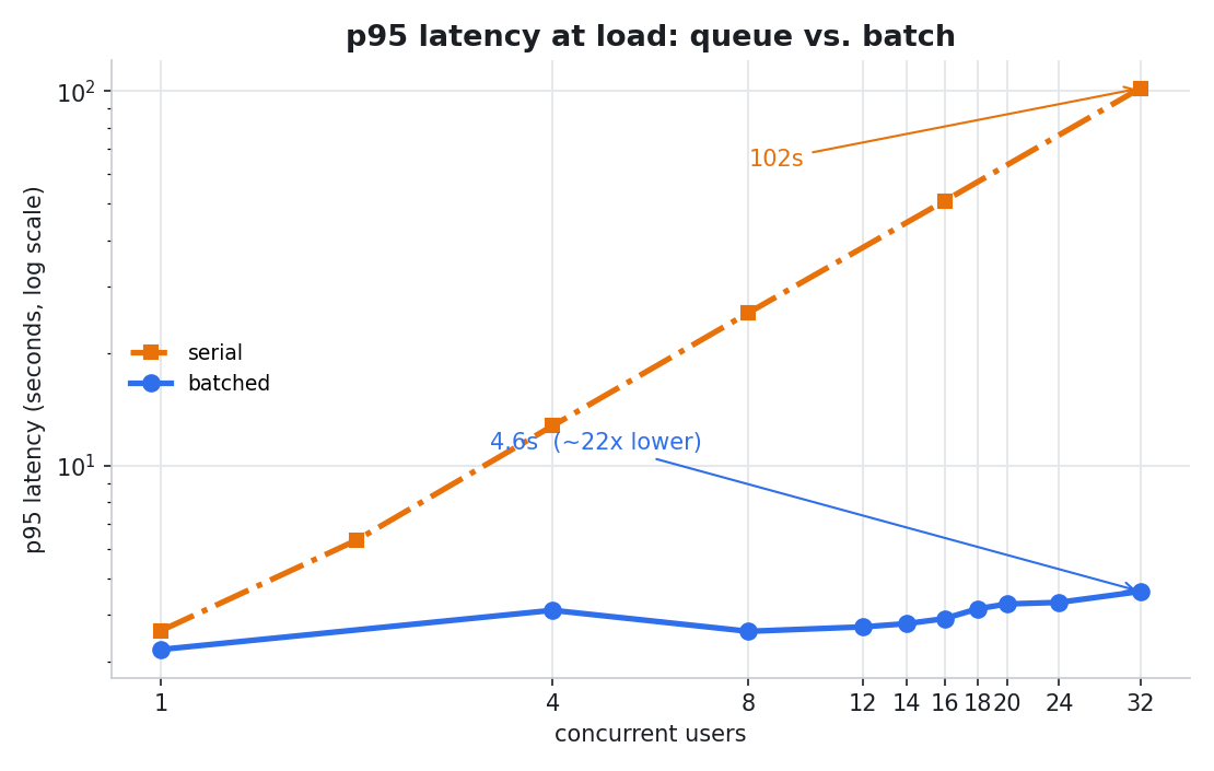
Latency alone would have shown that the endpoint was slow. Throughput alone would have shown that capacity was capped.

Viewed together, the curves showed that request-level concurrency was not becoming active inference work.

Ruling Out Client-Side Serialization

A flat throughput curve does not identify where the queue exists.

Possible explanations included:

• the load generator was serializing requests,
• the client connection pool was limiting parallelism,
• a local async lock or subprocess boundary was introducing a queue,
• the platform router was limiting in-flight requests,
• the replica accepted only one request at a time,
• the inference engine was constrained by its own scheduler settings.

To eliminate several client-local explanations, I launched independent operating-system processes at the same time.

Their completion times still formed a staircase: approximately 1x, 2x, and 3x the single-request service time.

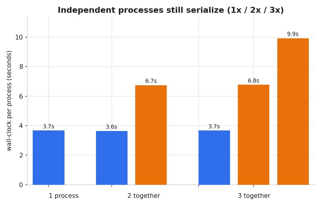
Independent processes do not share the same application-level async lock or local request queue. The test did not identify the exact remote admission-control layer, but it moved the suspected queue out of the client process and into the serving path.

That narrowed the investigation to the layers responsible for admitting concurrent requests to the engine.

Tracing Concurrency Through the Serving Path

vLLM can perform continuous batching, but the scheduler can only batch requests that reach it concurrently.

A deployed inference endpoint can constrain concurrency at several layers:

Layer	Diagnostic question
Client	Are requests actually issued concurrently?
Transport	Are connections, pools, or subprocesses serializing traffic?
Router	How many in-flight requests are directed to one replica?
Replica admission	How many requests can the container accept simultaneously?
Engine scheduler	How many sequences may remain active in a batch?
Autoscaler	Is scale-out obscuring single-replica capacity?

In this deployment, the critical controls were in the router and replica admission path: Baseten's production concurrency_target and the replica's runtime.predict_concurrency.

Once concurrent work was allowed through both layers, the engine could see enough simultaneous requests to batch them.

Engine capability and endpoint behavior are different properties.

One limitation: both admission controls were corrected as part of the successful intervention. That proves the serving-path hypothesis, but it does not isolate the individual contribution of each setting. A full factorial test would separately run low/low, high-router/low-replica, low-router/high-replica, and high/high.

The exact pre-engine queue was also inferred rather than directly observed. The platform metrics I captured after the fix showed scheduler-visible concurrency, but I did not capture historical router/replica queue-depth counters before the fix. The before-fix evidence is therefore: flat throughput, stair-stepped independent processes, and a controlled serving-path intervention that changed the curve.

The deployed vLLM configuration also matters for interpreting the result: prefix caching and chunked prefill were enabled, gpu_memory_utilization was 0.90, max_model_len was 4096, and max_num_seqs was 32. Chunked prefill lets long prompt processing be divided into smaller scheduling units so prefill work does not monopolize the batch; I did not independently isolate its contribution here.

Confirming Concurrency Propagation

After changing the serving-path admission controls, I repeated the concurrency sweep.

At 32 concurrent requests, throughput settled around 6.87 requests per second.

The result was measured across three runs of 150 requests each, with throughput coefficient of variation below 1%.

p95 latency fell from 102 seconds to approximately 4.6 seconds.

A later server-metrics scrape under 28 concurrent requests showed running=28 and waiting=0, consistent with concurrent work reaching the scheduler rather than waiting outside it.

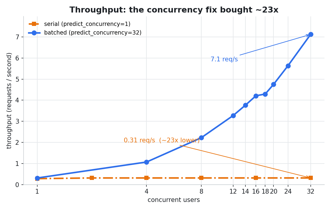
The evidence chain was:

load curve -> independent-process test -> admission-control hypothesis -> controlled serving change -> repeated sweep

The before-and-after curve showed that concurrent requests were now becoming active batched work.

The throughput improvement was approximately 22×.

Requests per second are useful, but token-normalized throughput makes the result more portable. At 6.87 requests/second and roughly 115 output tokens per request, the endpoint was producing about 790 output tokens/second. Multiplying request rate by logical prompt length gives approximately 22.7K presented input tokens/second. That is not equivalent to 22.7K newly computed prefill tokens/second because most shared prefix blocks were served from cache.

The more important result, however, was the diagnostic method: the serving change was tied to a measurable system hypothesis rather than applied as an unexplained configuration adjustment.

The Operating Knee and Saturation Point

Once concurrency propagation was working, the question changed from "does the endpoint scale?" to "where should it operate?"

Peak throughput is not automatically the best production target.

LLM serving commonly exhibits a knee: an operating range where throughput continues to improve efficiently, followed by a region where each additional concurrent request produces smaller throughput gains and higher tail latency.

The denser sweep showed that this endpoint scaled efficiently through approximately 16 concurrent requests, then began to bend.

Concurrency	Throughput	Scaling efficiency	p95 latency	Cost / 1k queries
1	0.31 req/s	100%	3.24s	$0.893
8	2.22 req/s	89%	3.62s	$0.125
16	4.21 req/s	85%	3.91s	$0.066
18	4.29 req/s	77%	4.16s	$0.065
24	5.63 req/s	75%	4.32s	$0.049
32	~6.87 req/s	~69%	~4.6s	~$0.04

Scaling efficiency was calculated as:

throughput at concurrency N / (N * single-request throughput)

Cost per 1,000 queries was calculated as:

hourly GPU cost / hourly completed requests * 1,000

For example, at concurrency 16, perfect linear scaling from the single-request baseline would have produced about 4.96 requests/second. The measured 4.21 requests/second therefore represents roughly 85% scaling efficiency.

The cost model used an assumed GPU price of $1 per hour. The absolute dollar figures should therefore be recalculated using the actual deployment price. The relative trend is the useful result.

Table note: the 16, 18, and 24 concurrency rows come from the denser knee sweep. The 32-concurrency row uses the more robust three-run variance result, so its efficiency is recomputed from ~6.87 req/s.

A later clean repeated sweep at 12, 16, 20, and 24 concurrent requests reinforced the same operating-range story:

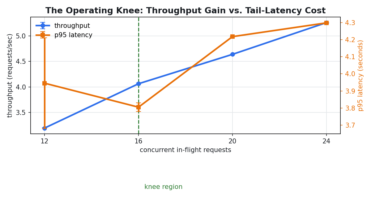
Concurrency	Throughput mean	p95 mean	Scaling efficiency
12	3.19 req/s	3.95s	86%
16	4.06 req/s	3.80s	82%
20	4.64 req/s	4.22s	75%
24	5.26 req/s	4.30s	71%

Two accidentally overlapped runs were excluded from this graph because they contended with each other.

An SLO, or service-level objective, turns that curve into a policy. For example:

Policy	Operating choice
p95 below 4 seconds	use the 16-request region
p95 below 4.5 seconds	use the 20-24 request region
lowest cost per query with p95 below 5 seconds	use the 32-request region

I also tested beyond 32 concurrent requests to separate the efficient operating knee from the endpoint's approximate saturation point.

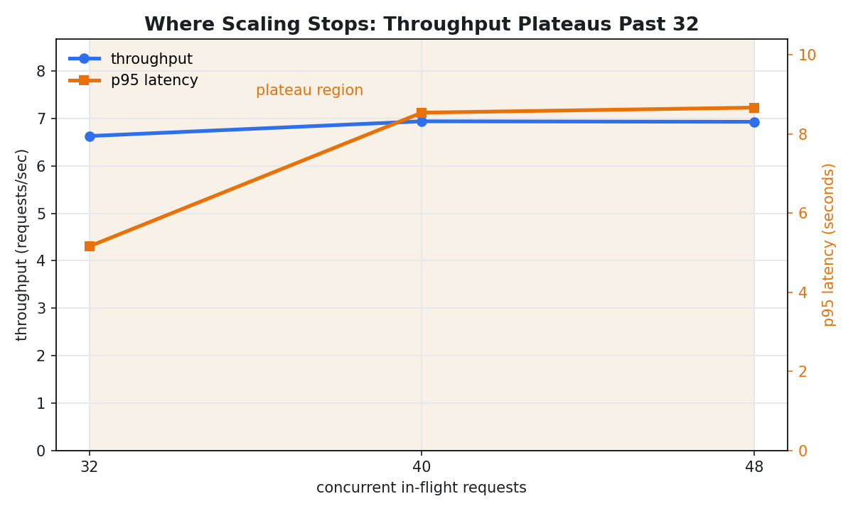
Concurrency	Throughput	p50	p95
32	6.63 req/s	4.37s	5.16s
40	6.94 req/s	4.44s	8.54s
48	6.93 req/s	4.57s	8.67s

Throughput plateaued around 6.9 requests/second while p95 jumped above 8.5 seconds. That suggests 32 was close to the practical single-replica capacity region for this workload, while 16 remained the cleaner SLO-first operating range.

The saturation sweep was a separate run and produced slightly different absolute values at concurrency 32. The canonical repeated measurement remains approximately 6.87 requests/second with sub-1% throughput variation; the beyond-32 sweep is useful for showing where additional concurrency stopped buying meaningful throughput.

A Long Prompt Is Cheap Only When Reusable

After the concurrency path was fixed, the next question was where request time was being spent.

LLM request latency is shaped by several components:

• Input sequence length, or ISL: the prompt and context processed by the model.
• Output sequence length, or OSL: the tokens generated by the model.
• Prefill: processing input tokens.
• Decode: autoregressively generating output tokens.
• Queue time: waiting before active execution.

The latency terms are worth naming precisely. TTFT means time to first token. Inter-token latency, sometimes discussed as time per output token, is the delay between generated tokens after output begins. Time to last token is the interval until generation finishes. For a non-streaming API, the user receives nothing until the full response is returned, so end-to-end response latency is the primary visible measure.

The real prompt in this workload was approximately 3.3K tokens because it contained schema and intent instructions.

A large prompt does not necessarily imply that prefill dominates latency.

Much of the prompt was shared across requests, allowing prefix caching to reuse previously computed KV blocks.

In the measured run, the prefix-cache hit rate was 99.6%.

That figure represents a best-case workload. The test repeatedly cycled the same 20 questions with a large shared prefix. A more diverse production stream would likely produce a lower hit rate.

For this workload, however, the warm shared prefix made repeated prefill inexpensive.

The following decomposition came from a sequential warm-prefix measurement. It should not be interpreted as the queue-time profile of the concurrent load sweep.

Component	Mean per request	Share of end-to-end
End-to-end latency	~3145 ms	100%
TTFT	~34 ms	~1%
Prefill time	~31 ms	within TTFT
Queue time	0 ms	sequential measurement
Decode time	~3110 ms	~99%
Inter-token latency	~27.2 ms/token	~37 tok/s
Output length	~115 tokens/request	-

In that warm-prefix measurement, decode accounted for nearly all measured request time.

That changed the optimization target.

Prompt length was no longer the dominant lever. Output length was.

The follow-up prefix experiments show why that conclusion has to stay scoped to the workload. The shared-prefix workload reproduced the best-case cache behavior. A deliberately diverse-prefix workload reduced the hit rate and moved latency back into TTFT and prefill:

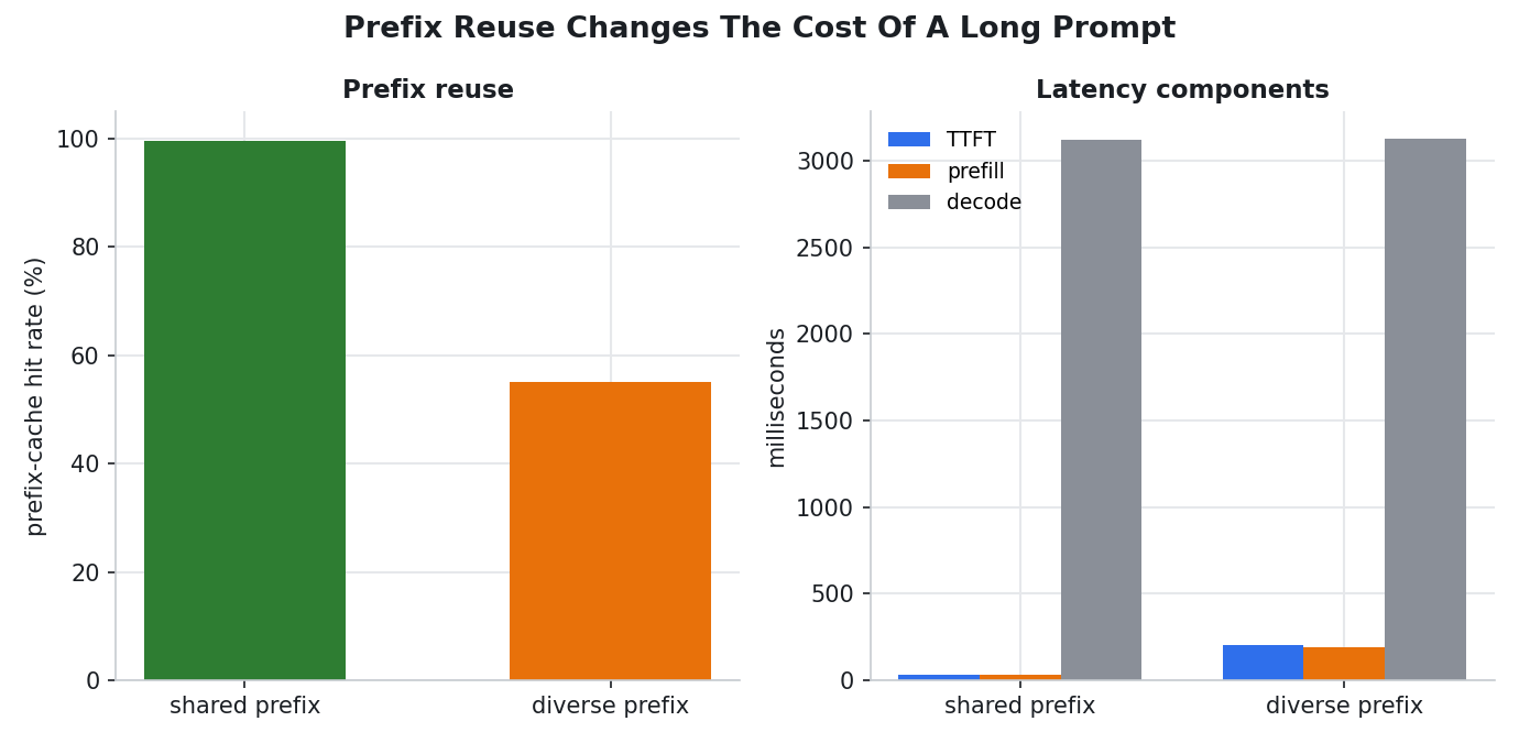
Workload	Prefix hit	TTFT	Prefill	Decode	Client p50
shared prefix	99.6%	34 ms	32 ms	3118 ms	3231 ms
diverse prefix	55.1%	206 ms	189 ms	3127 ms	3584 ms

Decode stayed roughly flat, while TTFT and prefill rose. A 3.3K-token prompt was cheap when the prefix was reusable, not because long prompts are generally cheap.

A second prefix-scenario run added a lower-reuse leading-unique prompt. It was colder than the shared-prefix runs, but not a zero-hit cold-cache test:

Scenario	Prefix hit	TTFT	Prefill	Client p50
warm shared prefix	99.6%	34-65 ms	32-44 ms	~3230 ms
partially shared prefix	99.3%	35 ms	32 ms	3232 ms
reduced-reuse leading-unique prompt	36.0%	280 ms	259 ms	3586 ms

The client-latency increase from shared to diverse or reduced-reuse prefix was larger than the server-reported prefill increase alone. I treat that exact delta as a mix of prefill, request-level timing, and metrics aggregation boundaries rather than forcing a single-cause explanation.

Output Tokens as a Latency Budget

The model emitted pretty-printed JSON at approximately 115 to 118 output tokens per request.

Compact JSON reduced that output to roughly 77 tokens in the live A/B test.

The expected latency savings could be estimated directly:

• Tokens saved: approximately 39.
• Inter-token latency: approximately 27.2 ms per token.
• Expected latency reduction: 39 * 27.2 ms ~= 1,060 ms.
• Measured reduction when compact output was honored: approximately 1,050 ms, or about 32%.

The close agreement between predicted and measured savings strengthens the causal explanation.

Decode time dominated the warm-prefix measurement, and reducing OSL reduced latency by the expected amount.

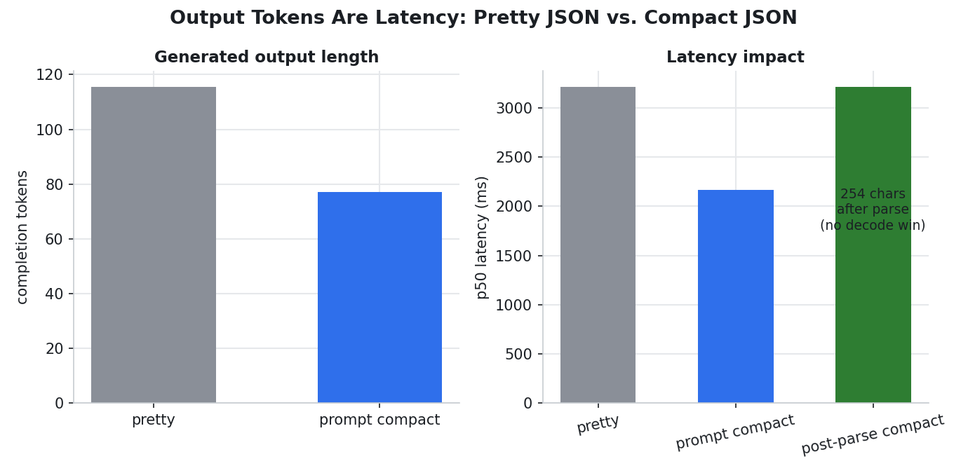
Output path	p50 latency	Completion tokens	Characters
pretty JSON	3214 ms	116	327
prompt-requested compact JSON	2169 ms	77	258
post-parse compact from pretty JSON	no decode win	n/a	254

The implementation lesson was equally important.

Prompting the model to minify JSON was not reliable, even at temperature 0. Sometimes the model complied, sometimes it did not, and sometimes the instruction increased output length.

In the live A/B, prompt-requested compact JSON was honored 7 of 12 times, ignored 4 times, and backfired once. The backfire increased output from 115 to 154 completion tokens and latency from 3199 ms to 4261 ms. The response still finished normally; it simply generated more text instead of less.

There are three different strategies, and they should not be conflated:

1. Prompt instruction can reduce generated tokens, but the model may ignore it.
2. Post-generation serialization deterministically reduces response bytes, but it cannot recover model decode time that has already been spent.
3. A generation-constrained compact grammar or representation can reduce decode latency by preventing unnecessary whitespace tokens from being generated in the first place.

By serializer-level enforcement, I mean compacting JSON in code after the model has produced a valid object. For example:

json.dumps(obj, separators=(",", ":"))

That reduces response bytes deterministically. It does not reduce model latency after the model has already generated pretty JSON. To reduce decode time, compactness has to be enforced before or during generation, through a structured-output grammar or serving layer that prevents whitespace-heavy JSON from being generated in the first place.

The production-grade latency solution is therefore not stronger wording in the prompt. Compactness has to be part of the generation contract, then measured again.

Context Budget as a Reliability Constraint

Output length also affected reliability through max_tokens.

With a 4,096-token context window, a prompt of approximately 3.3K tokens left enough headroom for max_tokens=256, but little room for uncontrolled prompt growth.

In an earlier run, a larger prompt combined with max_tokens=512 exceeded the context limit and returned an HTTP 400 before generation began.

Measuring actual output length turned max_tokens from a guess into an engineering decision:

• 128 tokens was tight.
• 256 tokens provided usable headroom.
• Every response path should still fail explicitly when finish_reason=length.

OSL was therefore both a latency variable and a context-budget constraint.

Ruling Out KV Pressure

The load curve exposed the serving symptom.

The token decomposition explained why decode mattered.

GPU and KV metrics helped rule out resource explanations.

Under a 28-concurrent-request load, the metrics export showed:

• GPU utilization: 78.5%.
• KV-cache usage: approximately 1.5%.
• vLLM running requests: 28.
• vLLM waiting requests: 0.
• GPU memory used: approximately 20.5 GB, reflecting vLLM's preallocated memory pool.
• Prefix-cache hit rate: 99.6% over the run.

The careful conclusion was:

KV capacity was clearly not the active constraint.

The remaining evidence was most consistent with decode-side execution, potentially limited by memory bandwidth, rather than KV capacity.

This was not a full roofline analysis. GPU utilization came from a coarse scrape, and decode workloads can be memory-bandwidth-bound without reporting 100% utilization.

The metrics were nevertheless sufficient to reject the wrong explanation: the endpoint was not limited by a full KV cache.

The low KV usage was also consistent with the model architecture.

Qwen2.5-3B uses grouped-query attention with two KV heads, reducing the cache footprint enough that a 32-request batch at the measured sequence lengths remained well below the available KV capacity of the 24 GB L4.

The complete system picture was therefore:

• Admission control determined whether requests reached the scheduler concurrently.
• Continuous batching improved throughput once the scheduler saw simultaneous work.
• Grouped-query attention kept KV pressure low.
• Prefix caching reduced repeated prefill cost.
• Decode dominated the warm-prefix request time.
• Output length became the next latency lever.

Performance Was Stable Under Load; Semantic Generalization Was Not

The serving results only matter if quality is not being traded away silently.

The complete pipeline produced the expected final result for all 20 development questions because deterministic correction and SQL generation handled the downstream path. Raw model intent accuracy on that same set was only approximately 75%.

The main error involved a narrow semantic distinction: whether "revenue by region" should be interpreted as a plain dimensional breakdown or a top-N ranking. Structured decoding addressed output shape, not semantic reasoning; once the request used the correct vLLM 0.12.0 field, structured_outputs, JSON schema compliance became reliable, but the model's ranking-versus-breakdown decision did not improve.

A deterministic one-way guardrail corrected the unsupported ranking case on the tuned set. Quality under load was also tested directly: at concurrency levels 1, 16, and 32, the raw intents were bit-identical for this workload.

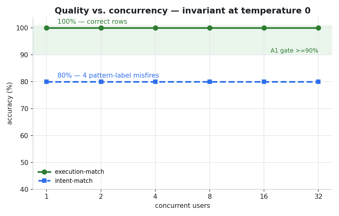
The harder question was whether that quality result generalized. A held-out semantic evaluation means testing on questions that were not used while developing the prompt, guardrail, schema, or examples. This run used a larger semantic holdout and reported raw intent accuracy, corrected system accuracy, intervention count, and intervention precision separately.

A contrastive prompt teaches the model by placing two similar-looking questions next to each other and explaining the difference. For example, "revenue by region" asks for a breakdown, while "top regions by revenue" asks for a ranking. Both mention revenue and region; the word "top" changes the operation. On the held-out set, however, this improved raw accuracy by only 1.6 percentage points.

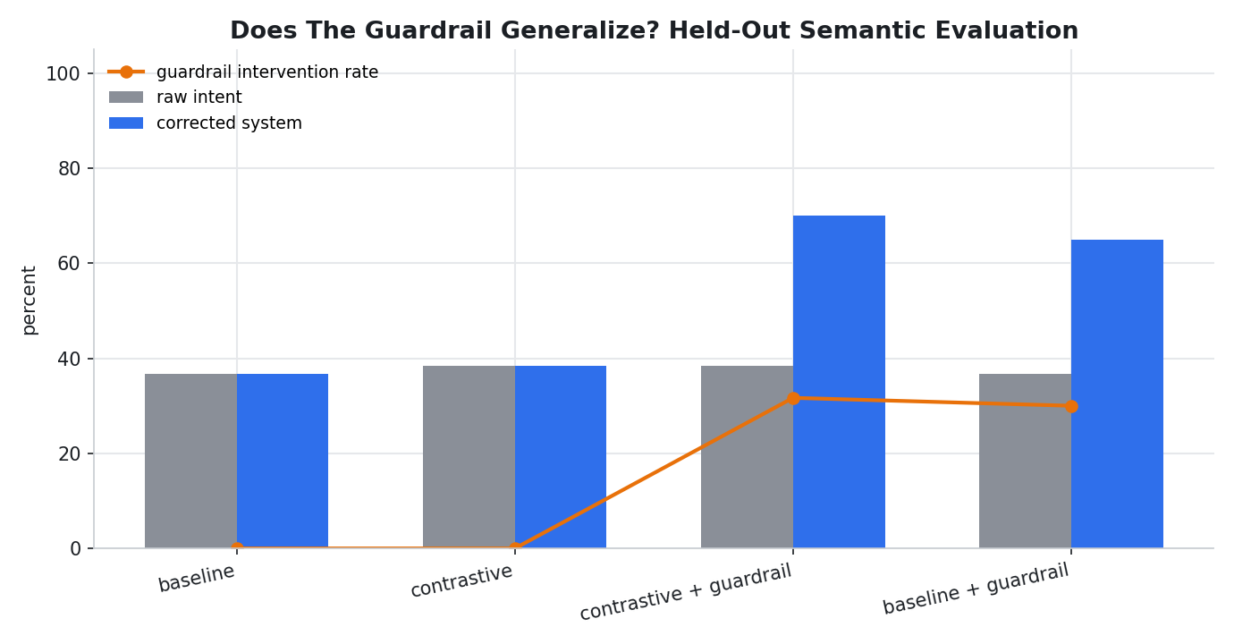
Condition	Raw intent	Final accuracy after guardrail	Interventions	Precision
baseline	36.7%	36.7%	0	n/a
contrastive prompt	38.3%	38.3%	0	n/a
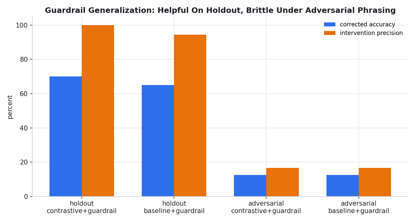
contrastive + guardrail	38.3%	70.0%	19	100.0%
baseline + guardrail	36.7%	65.0%	18	94.4%

Intervention precision measures whether the guardrail was correct when it changed the model's answer. It does not measure overall system accuracy.

The 19 correct interventions did not produce 100% final accuracy because the remaining errors involved fields outside the guardrail's scope, including limits, filters, sorting, and other intent patterns.

This is the most important correction to the quality story. The guardrail generalized partially and with high intervention precision, but the held-out semantic gate was not solved. The serving conclusions still stand, but the quality claim should remain scoped: the tuned 20-question pass was an engineering checkpoint, not a generalization result.

The held-out set was intentionally challenge-heavy rather than a random production sample: 40 contrast-pair questions plus 20 naturalistic questions, with an expected-label distribution of 30 breakdown, 27 top-N ranking, and 3 time-series questions. The majority-class baseline was therefore 50%.

The baseline model's main raw error was false ranking: it often interpreted a plain breakdown as top_n_by_metric. On the contrastive+guardrail condition, the guardrail corrected 19 of 19 raw false-ranking cases. For that observed error category on this holdout, it had 100% recall and 100% precision.

That does not mean the guardrail was robust. I also ran a small adversarial phrasing set:

Phrase	Superficial cue	Actual meaning
"top-line revenue by region"	contains "top"	"top-line" means revenue, not ranking
"first ten rows"	contains a limit	row count does not necessarily mean top-N
"regions leading in revenue"	no word "top"	still expresses ranking
"revenue by region, descending"	sort cue	may request sorting, not top-N truncation

On that adversarial set, both guardrail conditions had only 16.7% intervention precision. The guardrail was useful for the observed false-ranking cluster, but it was still too lexical and brittle for broad semantic generalization.

A Control-to-Signal Map

The most reusable operational habit from the investigation was pairing every control with a measurable signal.

Control or design choice	Expected effect	Signal to watch
Client concurrency	Whether traffic is issued concurrently	Client timestamps, wall time, connection-pool behavior
Router admission	Whether in-flight requests reach one replica	Replica count, router queueing, per-replica concurrency
Replica admission	Whether the container accepts concurrent requests	Throughput curve, active requests
Engine batch limits	Maximum number of active sequences	Running requests, waiting requests, KV usage
Prefix caching	Reuse of shared prompt KV	Cache-hit rate, TTFT, prefill time
ISL	Prefill cost and context consumption	Prompt tokens, TTFT, cache-hit rate
OSL	Decode time and response size	Completion tokens, inter-token latency, decode time
max_tokens	Truncation risk and context headroom	Finish reason, token count, parse failures
max_model_len	Context capacity and KV allocation	Context errors, KV usage, batch knee
Structured outputs	Schema compliance	Parse errors, finish reason, schema validity
Semantic guardrails	Correct targeted error clusters	Intervention precision, intervention recall, adversarial phrasing tests
Held-out evaluation	Test generalization beyond tuned examples	Raw intent accuracy, final accuracy after correction, error taxonomy
Model architecture	KV footprint and per-token performance	KV usage, tokens per second, cost per query

This converts performance tuning into a falsifiable loop:

1. Change one control.
2. Predict which signal should move.
3. Measure whether it moved.
4. Reject explanations that do not match the evidence.

Conclusion

Continuous batching is not something an inference engine delivers by itself.

It is an end-to-end system behavior that depends on whether concurrent requests survive the serving path and arrive at the scheduler together.

The practical lesson is to treat an LLM endpoint as a system, not as a model behind an API.

Production LLM systems have at least three independent control planes. Infrastructure controls how efficiently work reaches the GPU. Structured output controls the shape of the answer. Semantic evaluation determines whether the answer means the right thing. Continuous batching solved the first problem. Structured decoding helped with the second. The held-out and adversarial results show the third is still open.

Plot the curves.

Trace admission control.

Measure the tokens.

Read the GPU.

Then choose the operating range with evidence.

Part 2: From Serving Correctness To Production Intelligence

The serving investigation fixed one control plane: whether concurrent requests reached the GPU scheduler as batched work.

It did not solve every production question around this NLQ2SQL system. In fact, the follow-up runs made the next layer clearer. The endpoint could be made fast and measurable, but semantic generalization, model routing, context sizing, multi-replica scheduling, and autoscaling policy still needed their own evidence.

That is the next article I would write.

The Next Quality Gate

The held-out semantic evaluation changed the quality story.

The original 20-question set was useful as an engineering checkpoint, but it had already influenced the prompt and guardrail design. On the larger challenge-heavy holdout, final accuracy after guardrail reached 65-70%, below the >=90% target I would want before calling the task solved.

That creates a more interesting question than "should I use a bigger model?"

The question is:

Which intervention buys semantic correctness most efficiently?

I would compare several systems on the same development, held-out, and adversarial sets:

Candidate	What it tests
3B baseline	The current raw model reference point.
3B + current guardrail	The current transparent correction layer.
3B + refined guardrails	Whether deterministic invariants can expand without false positives.
3B + planner or clarifier	Whether decomposing the user question beats direct intent generation.
7B baseline	Whether more local/open-model capacity improves raw semantics.
7B + guardrail	Whether a larger model plus transparent correction is enough.
Claude Haiku-class model	A hosted latency/cost comparison through Bedrock or direct API.
Claude Sonnet-class model	A hosted stronger-reasoning comparison through Bedrock or direct API.
OpenAI small model	A hosted cost-sensitive comparison.
OpenAI stronger model	A hosted quality-ceiling comparison.

The important part is that every candidate should be scored the same way:

Metric	Why it matters
Raw intent accuracy	Measures model semantics before correction.
Final accuracy after guardrail or planner	Measures system quality.
Intervention precision	Measures whether corrections are safe when they fire.
Intervention recall	Measures whether corrections catch the intended error class.
Error taxonomy	Shows whether failures are one cluster or many.
p50/p95 latency	Keeps quality wins tied to serving cost.
Output tokens	Explains latency and API cost differences.
Cost per 1,000 questions	Turns model choice into an operating decision.

If a 7B model meaningfully improves raw intent accuracy, it may simplify the system. If a planner or clarifier gets the 3B model near the quality gate, that may be cheaper and easier to operate. If hosted frontier models produce the quality ceiling, they become the benchmark for whether the local stack is worth further optimization.

Context Window Sizing Is Capacity Planning

The context-window question looks simple from the outside: if 4K is tight, why not use 8K?

But in serving, context length is also a capacity variable. A larger max_model_len can change memory reservation, KV-cache planning, maximum batch shape, and the operating knee. The right move is not to maximize the window by default. It is to measure the actual input sequence length, output sequence length, and headroom requirement.

For this workload, the prompt was about 3.3K tokens and the output was usually around 115-118 tokens. max_tokens=256 gave enough output headroom on a 4,096-token deployment, while an earlier larger prompt plus max_tokens=512 exceeded the context limit before generation began.

The sizing workflow should be:

1. Measure actual ISL and OSL.
2. Choose max_tokens from observed valid outputs plus growth margin.
3. Raise max_model_len only when a real prompt-growth requirement exists.
4. Re-run the knee sweep after changing it.
5. Watch context errors, KV usage, p95 latency, and throughput.

The experiment I would run next is simple:

max_model_len=4096 versus max_model_len=8192
same prompt
same output contract
same concurrency sweep
same quality set

If the 8K setting preserves the knee and leaves KV pressure low, it buys future schema headroom. If it moves the knee down or worsens p95, it is not free.

Multi-Replica Routing Is Not Just Round Robin

The single-replica experiment answered one question: how much work one L4-backed endpoint could absorb for this workload.

A production system also has to decide how requests should be distributed across replicas.

Round-robin is attractive because it is simple. But it can create hot workers when requests are not equal. Two requests can have the same API shape and very different serving cost because they differ in input length, output length, cache reuse, or decode duration.

A better router might consider:

Signal	Why it helps
In-flight requests per replica	Avoids sending work to a busy replica.
Estimated input tokens	Predicts prefill cost and context pressure.
Estimated output tokens	Predicts decode occupancy.
vLLM running and waiting requests	Shows scheduler pressure directly.
Prefix-cache affinity	Preserves reuse for shared schemas or tenants.
Recent p95 latency	Captures tail behavior better than averages.
GPU utilization	Shows execution pressure.
KV-cache usage	Shows memory pressure and batch headroom.

There is a real tradeoff here:

Routing for balance can hurt prefix-cache reuse. Routing for cache affinity can create hot workers.

That means the router needs a policy, not a slogan. A reasonable first policy is a weighted score that considers current load, estimated token work, and prefix affinity together.

Autoscaling Should Follow SLO Pressure

Autoscaling on request count alone is too blunt for LLM serving.

The endpoint should scale based on the service objective:

Mode	Primary objective	Scaling signal
Latency-first	Keep p95 below target	p95 latency, queue time, waiting requests
Cost-first	Minimize cost per successful query	throughput per replica, utilization, cost/query
Throughput-first	Maximize completed work	tokens/sec, saturation plateau, queue growth
Quality-first	Route hard questions correctly	semantic confidence, model tier, correction risk

Cold start time has to be part of that model. If a sleeping replica takes roughly two minutes to become useful, scale-out cannot wait until the SLO is already broken. The system needs to pre-warm capacity when the current slope of traffic predicts a future breach.

The architectural question becomes:

Given current load, queue growth, p95 latency, and replica startup time,
when should the system add capacity?

That is a more realistic production problem than choosing a single concurrency number.

The Bigger Lesson

Part 1 showed that request concurrency only matters if it becomes scheduler-visible batched work.

Part 2 extends that idea:

Production LLM behavior is controlled by several interacting policies: semantic routing, context budgeting, request admission, replica routing, batching, autoscaling, and model selection.

Each policy needs a signal. Otherwise, the system looks operational because it has knobs, but the knobs are not tied to evidence.

Caveats

• The canonical throughput result is approximately 6.87 requests per second, or roughly 22× the original throughput, based on three 150-request runs with throughput coefficient of variation below 1%.
• The full system passed a fixed 20-question test that had already influenced development, but the live held-out semantic evaluation reached only 65-70% corrected system accuracy depending on prompt/guardrail condition.
• The semantic holdout was challenge-heavy and should not be treated as a random sample of production traffic.
• The adversarial phrasing test showed the current guardrail is brittle; it helped the held-out false-ranking cluster but is not a complete semantic solution.
• KV capacity was ruled out as the active constraint. The remaining evidence was most consistent with decode-side execution, potentially limited by memory bandwidth, but this was not a full roofline analysis.
• The 99.6% prefix-cache hit rate is a best-case result from repeatedly cycling 20 prompts with a shared prefix.
• The cost calculation assumes an L4 price of $1 per hour.
• The compact-JSON A/B produced the expected latency reduction only when the model honored the format. Client-side post-parse compacting reduces bytes but not decode time; latency reduction requires generation-time or serving-layer enforcement.

Reproducibility Note

All reported measurements came from retained JSON run artifacts, server-metrics captures, generated plots, and reproducible analysis scripts. The vLLM structured-output API detail was checked against the official documentation: https://docs.vllm.ai/en/latest/features/structured_outputs/.