
Part 6 — Inference Fundamentals
Inside an NVIDIA GPU: a visual tour
Build an accurate visual model of SMs, Tensor Cores, warps, and the local memory hierarchy—then use measurements rather than slogans to diagnose LLM inference.
“Prefill is compute-bound” and “decode is memory-bound” are useful starting hypotheses—not hardware laws. This chapter draws the GPU, then shows how arithmetic intensity, workload shape, kernels, and measured counters determine which resource actually limits an inference phase.
What you will understand by the end
- How CPU and GPU design priorities differ.
- The hierarchy from GPU → streaming multiprocessor (SM) → execution pipelines.
- Which memory is local, which storage is software-managed, and which paths are remote.
- Why occupancy, activity, and utilization are different metrics.
- How to test common prefill and decode bottleneck hypotheses.
CPU versus GPU: two different priorities
A latency-oriented CPU core spends substantial silicon on control, prediction, and cache to accelerate a small number of instruction streams. A GPU devotes more of the chip to many lightweight execution contexts and parallel arithmetic. Compared with a CPU core, a GPU thread relies more on concurrency than strong single-thread execution.
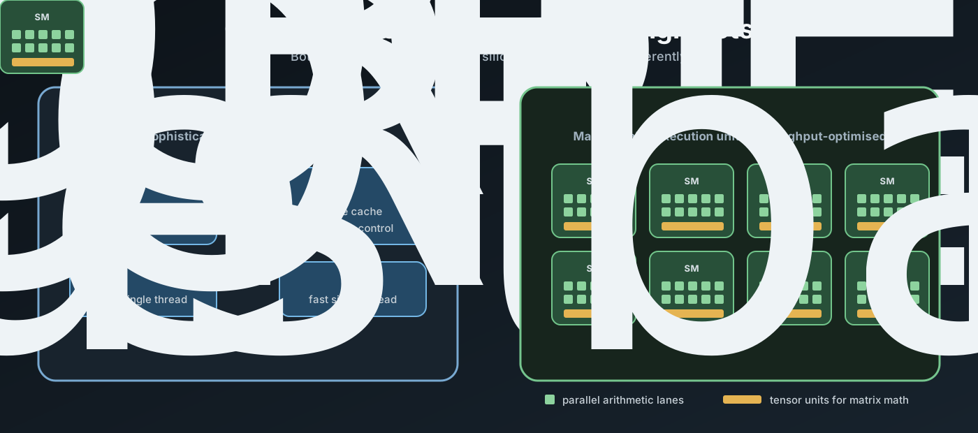
A GPU excels when a problem exposes enough regular, independent work. Transformer matrix operations often do; small or irregular kernels may not.
The die: an array of SMs
An NVIDIA GPU contains many streaming multiprocessors connected through on-chip cache, interconnect, and memory resources. Counts vary by die and SKU: the full GH100 design contains 144 SMs, H100 SXM5 enables 132, and H100 PCIe enables 114. “H100” alone is not a complete hardware specification.

Inside an SM:
- General-purpose execution pipelines handle scalar/vector arithmetic, address calculations, control-heavy operations, and elementwise work. FP, integer, load/store, and special-function organization varies by architecture.
- Tensor Cores accelerate supported matrix operations. Large projections and MLP GEMMs often use them, but an inference step also includes normalization, attention, reductions, sampling, memory traffic, launches, and sometimes communication.
- Warp schedulers, registers, shared memory, and L1 keep many threads supplied with instructions and data.
The largest AI throughput figures on a data-center GPU specification usually describe Tensor Core operations at a stated precision and may assume sparsity. Read the precision, density, clock, and methodology attached to every FLOPS or TOPS number.
Hopper introduced FP8 Tensor Core acceleration; Blackwell adds native FP4-class support such as NVFP4. Lower precision raises peak matrix throughput only when the hardware, kernel, model, and shapes support that execution path.
Vendors may disable units to salvage dies or segment products, but model numbers do not form a dependable “same die plus more enabled cores” ladder. Compare the exact SKU’s SMs, memory subsystem, precision support, power envelope, form factor, and interconnect.
Local memory hierarchy versus remote paths
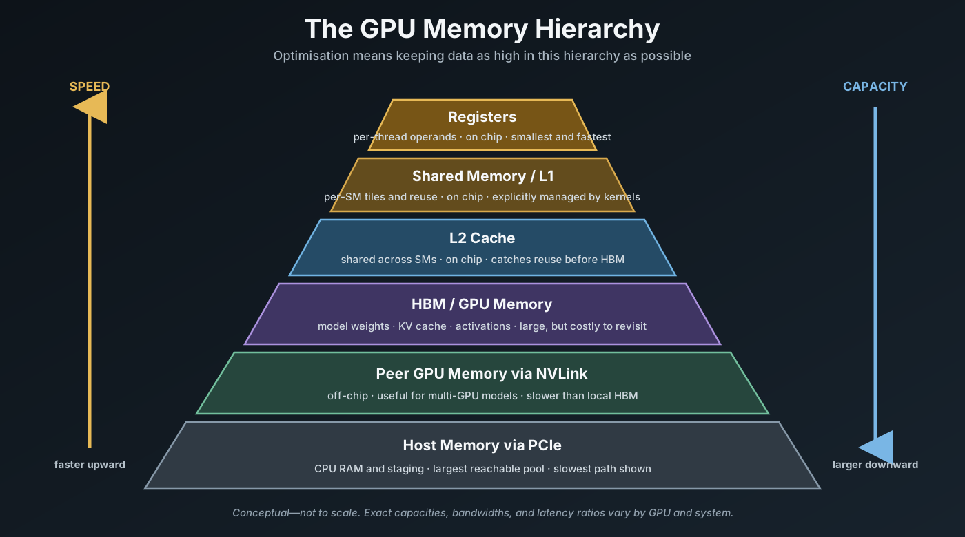
- Registers hold per-thread values.
- Shared memory is allocated and addressed explicitly by a thread block. Threads in the block can exchange tiles through it and synchronize.
- L1 is hardware-managed caching. On modern architectures, L1 and shared memory may share physical capacity or a configurable carveout, but their semantics differ.
- L2 is shared across the GPU and can retain data reused across SMs.
- Local HBM or GDDR normally holds weights, KV state, activations, and workspaces.
On-chip storage offers much lower latency and much higher aggregate bandwidth than local device memory. Exact ratios depend on architecture and access pattern, so reason from measured latency, achieved bandwidth, coalescing, cache behavior, and reuse—not one universal multiplier.
Capacity determines what combination of weights, KV state, activations, workspaces, communication buffers, graph captures, and concurrency can reside. Bandwidth constrains how quickly memory traffic can be served. Context, batch, architecture, cache behavior, and compute make both relevant to more than one inference phase.
FlashAttention is a useful memory-hierarchy example: it tiles exact attention so it does not materialize the full score matrix in HBM. Registers and shared memory retain working tiles, reducing expensive device-memory traffic even though the required attention result is unchanged.
Warps, blocks, and occupancy
Threads execute in warps of 32. Thread blocks contain one or more warps; a block is assigned to one SM for its lifetime, and an SM may host multiple blocks when register, shared-memory, and architectural limits allow. Divergent branches can serialize paths before reconvergence; newer independent-thread scheduling improves flexibility but does not make divergence free.
Occupancy is the fraction of an SM’s maximum warp slots that are resident for a kernel. More resident warps can help hide instruction or memory latency by giving the scheduler other ready work, but high occupancy is neither necessary nor sufficient for high performance. Registers and shared-memory use may intentionally trade occupancy for more useful work per thread.
| Metric | What it means |
|---|---|
| Occupancy | Resident warps relative to the hardware maximum for a kernel |
| SM activity | Cycles or time with active SM execution; exact denominator depends on the counter |
| Tensor activity | Cycles in which Tensor Core instruction pipes are active |
NVML / nvidia-smi GPU utilization |
Percentage of the sample interval during which one or more kernels executed |
“The GPU was 80% utilized” is not a hardware diagnosis unless the counter, sample interval, and denominator are specified. Kernel-active time does not reveal SM saturation, Tensor Core throughput, memory stalls, or useful-work efficiency.
Roofline reasoning: operations per byte
The useful bridge from the picture to performance is arithmetic intensity:
arithmetic intensity = useful operations ÷ bytes moved
A kernel with high arithmetic intensity may approach a compute ceiling. A low-intensity kernel is more likely to approach a memory-traffic ceiling. Actual position depends on shapes, batch, cache state, precision, kernel implementation, communication, and the target GPU’s compute-to-bandwidth balance.
| Regime | Common behavior | Important exceptions |
|---|---|---|
| Long, uncached dense prefill | Often compute-heavy | Short input, cached-prefix extension, MoE, communication, poor kernels |
| Low-batch dense decode | Often weight- or KV-traffic dominated | Launch gaps, CPU starvation, long-KV attention, communication, poor kernels |
| Higher-batch decode | Greater arithmetic intensity and weight-tile reuse | Attention/KV traffic, latency limits, or communication may dominate |
| Short extension after a prefix-cache hit | Little new prefill work | Reading the existing KV state can resemble decode behavior |
Batching adds independent work and often turns narrow matrix-vector-like decode into larger matrix operations. It can improve Tensor Core shapes, amortize launches and scheduling, and reuse loaded weight tiles across more activation rows. It does not guarantee that every weight is read once for the whole batch, and gains depend on the kernel, scheduler, sequence state, and latency objective.
For low-batch, dense, weight-traffic-dominated decode, a rough lower bound is:
step time ≥ bytes moved per step ÷ achieved memory bandwidth
Model-weight bytes may dominate that estimate, but KV traffic, scale metadata, dequantization, intermediates, communication, cache reuse, and non-overlapped overhead must be included before treating it as a prediction.
Quantization can reduce model footprint and memory traffic. It increases matrix throughput only when a validated low-precision kernel maps efficiently to the target architecture; conversion or dequantization can erase part of the gain.
How to prove a bottleneck
Start with request-level TTFT, inter-token latency, throughput, queueing, and batch shape. Then connect them to engine and kernel evidence:
- achieved DRAM and L2 throughput;
- SM and Tensor Core activity with exact counter definitions;
- kernel duration, launch gaps, synchronization, and CPU/GPU timeline;
- arithmetic intensity or roofline position;
- occupancy, eligible warps, and stall reasons;
- controlled changes to batch, precision, clocks, or bytes moved.
Use an execution timeline such as Nsight Systems, then architecture-specific counters and roofline analysis in Nsight Compute. A controlled intervention is stronger evidence than one generic percentage.
In this project’s single-L4 experiment, KV-cache occupancy remained near 1.4% in the observed range while requests continued scaling without queueing at 24 users. That establishes KV-capacity headroom—not the limiting execution resource. Distinguishing Tensor Core, DRAM-bandwidth, launch, or kernel-efficiency limits requires defined counters, kernel timing, or a controlled roofline-style intervention. Read the serving-knobs experiment →
Practical guidance
- Treat precision-specific Tensor Core throughput as a compute ceiling for compatible kernels, memory bandwidth as a traffic ceiling, capacity as the fit/concurrency envelope, and interconnect as a multi-GPU constraint.
- Treat software and kernel support as the condition for reaching any theoretical path.
- Form a bottleneck hypothesis from the workload, then confirm it with named metrics.
- Rebenchmark after changing model, context, batch, precision, kernel, topology, or GPU.
Summary
- NVIDIA GPUs contain arrays of SMs; exact resources vary by architecture and SKU.
- Tensor Cores supply matrix throughput, but end-to-end inference uses the whole system.
- The local hierarchy ends at HBM/GDDR; peer and host memory are remote access paths.
- Occupancy, SM activity, Tensor activity, and NVML utilization are different quantities.
- Prefill and decode have common operating regimes, not universal bottlenecks.
- Diagnose performance with arithmetic intensity, timelines, counters, and interventions.
Knowledge check
Decode is slow, memory capacity is mostly free, and nvidia-smi reports low utilization. What can you conclude?
You can rule out simple device-memory exhaustion. You cannot identify the performance limiter. Check offered load and queueing, then inspect achieved DRAM/L2 throughput, SM and Tensor activity, launch gaps, kernel duration, batch shape, and KV traffic. If evidence confirms low-batch weight-traffic dominance, batching or quantization may help; otherwise match the intervention to the measured limiter.
Why can a high-occupancy kernel still be slow?
Occupancy counts resident warps, not useful instructions or resource saturation. Those warps may all stall on memory, execute inefficient instructions, or compete for another resource. Conversely, a lower-occupancy kernel may use registers effectively and saturate its limiting compute or bandwidth resource.
Why is FlashAttention a memory-hierarchy optimization?
It computes exact attention while tiling work through registers and shared memory so the full score matrix is not written to and read from HBM. The gain comes from reduced high-cost data movement, not from making attention approximate.
Primary sources and version boundary
Hardware and tooling claims were reviewed August 2, 2026. Always verify the exact GPU, driver, CUDA, library, and profiler versions used in a measurement.
- CUDA C++ Best Practices: occupancy
- NVML utilization definition
- NVIDIA Hopper architecture and H100 SKU SM counts
- CUDA Programming Guide: memory hierarchy
- NVIDIA Blackwell architecture and NVFP4
- NVIDIA long-context inference regimes
- Nsight Systems and Nsight Compute
- FlashAttention: IO-aware exact attention